Week 2: Training Linear Classifiers & The XOR Problem
Accompanying Notebooks:
![]()
Click File -> Save a copy in Drive
Summary:
In this module, you will:
- Implement the perceptron learning algorithm
- Visualize how decision boundaries evolve during training
- Understand the mathematical foundation of weight updates
- Discover why some problems require deeper networks
- Understand how multi-layer perceptrons makes it possible to solve non-linearly separable problems
Introduction
In Week 1, you manually adjusted weights using sliders to find decision boundaries. But manual tuning would be impossible if you had thousands or millions of weights. This week, we’ll learn how computers can automatically find optimal weights through the perceptron learning rule.
Section 3.1: The Perceptron Model
Mathematical Foundation
The perceptron makes predictions using the same linear model from Week 1, but now we’ll see how to train it automatically.
Prediction Formula:
\[\hat{y} = \text{sign}(w \cdot x + b)\]Where:
- $x = [x_1, x_2]$ is the input vector (our 2D coordinates)
- $w = [w_1, w_2]$ are the weights (learnable parameters)
- $b$ is the bias (also learnable)
- $\hat{y}$ is the predicted class: $+1$ or $-1$
The sign function returns $+1$ if its input is non-negative, and $-1$ otherwise. This creates a hard threshold at zero.
Alternative Formulation:
You might also see this written as:
\[\hat{y} = \begin{cases} +1 & \text{if } w_1x_1 + w_2x_2 + b \geq 0 \\ -1 & \text{if } w_1x_1 + w_2x_2 + b < 0 \end{cases}\]Both formulations are equivalent - the perceptron checks which side of the decision boundary a point lies on.
Geometric Interpretation
Remember from Week 1 that $w_1x_1 + w_2x_2 + b = 0$ defines a line. The perceptron uses this line as its decision boundary:
- Points above/on the line: classified as $+1$
- Points below the line: classified as $-1$
In our examples, we label the $+1$ region as $blue$ and the $-1$ region as $red$.
The weight vector $w = [w_1, w_2]$ is perpendicular to the decision boundary. This geometric fact will be crucial for understanding how the learning algorithm works.
Section 3.2: The Perceptron Learning Rule
How Does Learning Work?
The steps of how a perceptron learns are as follows:
- Initialize weights and bias to some random small values
- Train a Epoch: one pass through all of the data:
- For each data point (iteration):
- Make a prediction
- If the prediction is wrong, update the weights
- If the prediction is correct, do nothing
- For each data point (iteration):
- Repeat Step 2 for multiple epochs (until there are no errors or a limit is reached).
Vocab:
- Iteration: Updating weights for a single example
- Epoch: Updating weights after seeing every example in the dataset once
The Update Rule
When the perceptron makes a mistake on input $x_i$ with true label $y_i$:
\[w_{\text{new}} = w_{\text{old}} + \alpha \cdot y_i \cdot x_i\] \[b_{\text{new}} = b_{\text{old}} + \alpha \cdot y_i\]Where:
- $\alpha$ is the learning rate (typically 0.1 or 0.01), which adjusts the magnitude of the update step.
- $y_i \in {-1, +1}$ is the true label
- $x_i$ is the input that was misclassified
Note: The Learning Rate Trade-off
The learning rate ($\alpha$) controls how drastically we change the weights:
- If too large: The model becomes unstable. The decision boundary swings wildly, potentially “overshooting” the solution and un-learning previous correct classifications.
- If too small: The model learns too slowly. It requires thousands of epochs to move the boundary to the correct place.
Example:
Suppose we have a blue point (label $y_i = +1$) at position $x_i = [1, 1]$, but our perceptron incorrectly predicts $-1$ (red).
This means $w \cdot x_i + b < 0$ when it should be $\geq 0$. We need to increase the score $w \cdot x_i + b$.
By the update rule: \(w_{\text{new}} = w_{\text{old}} + \alpha \cdot (+1) \cdot [1, 1] = w_{\text{old}} + \alpha [1, 1]\)
This adds a positive contribution in the direction of $x_i$, which increases $w \cdot x_i$.
Conversely: If we mistakenly predict $+1$ for a red point (true label $-1$), we multiply by $-1$, which subtracts from $w$, decreasing the score.
Why are we changing the labels from {0, 1} to {-1, +1} in our code?
The perceptron algorithm requires labels to be {-1, +1} instead of the more intuitive {0, 1}.
The Mathematical Reason:
Recall the update rule when we make a mistake:
\[w_{\text{new}} = w_{\text{old}} + \alpha \cdot y_i \cdot x_i\]The label $y_i$ acts as a direction multiplier:
- When $y_i = +1$ (blue point): we add $+\alpha x_i$ to the weights
- When $y_i = -1$ (red point): we add $-\alpha x_i$ to the weights
What would happen with {0, 1} labels?
If we used $y_i \in {0, 1}$:
- When $y_i = 1$: update works → $w \leftarrow w + \alpha \cdot 1 \cdot x_i$
- When $y_i = 0$: no update → $w \leftarrow w + \alpha \cdot 0 \cdot x_i = w$
Multiplying by zero produces no weight change for Class 0 misclassifications. The algorithm would only correct mistakes on Class 1 points, making it unable to learn the correct boundary.
Why {-1, +1} works:
With signed labels, both classes contribute to learning:
- Class 1 mistakes ($y_i = +1$): push the boundary toward the misclassified point
- Class 0 mistakes ($y_i = -1$): push the boundary away from the misclassified point
The negative sign for Class 0 encodes the “opposite direction” we need to move the decision boundary.
In Practice:
Since most datasets use {0, 1} labels naturally (like our OR and XOR gates), we convert them before training:
# Convert 0 labels to -1, leave 1 labels as is
y_signed = np.where(y == 0, -1, 1)
Geometric Interpretation of Updates
When we update $w \leftarrow w + \alpha y_i x_i$, we are actually rotating the decision boundary. Hopefully you’ve noticed this in week 1’s module.
- If we misclassify a blue point ($y_i = +1$), we rotate the boundary toward that point
- If we misclassify a red point ($y_i = -1$), we rotate the boundary away from that point
The learning rate $\alpha$ controls how much we rotate per mistake. Smaller $\alpha$ means slower, more careful learning.
Section 3.3: Training Dynamics on the OR Gate
Why OR is Linearly Separable
Recall the OR gate truth table:
| $x_1$ | $x_2$ | OR Output |
|---|---|---|
| 0 | 0 | 0 |
| 0 | 1 | 1 |
| 1 | 0 | 1 |
| 1 | 1 | 1 |
Observing Training
When you run the perceptron on OR in the notebook, you’ll see:
- Early epochs: The boundary is random, making many mistakes
- Middle epochs: The boundary rotates toward the correct orientation
- Later epochs: The boundary stabilizes, correctly separating all points
The color gradient visualization (purple → yellow) shows this progression beautifully. Notice how the boundary “settles” into a valid position.
Typical Convergence: OR gate usually converges in 5-10 epochs with learning rate 0.1, though this varies with initialization.
Sample gif of training:
Section 4.1: Why XOR is Not Linearly Separable
The XOR Problem
XOR is true when inputs are different.
Here’s the truth table again as a refresher:
| $x_1$ | $x_2$ | XOR Output |
|---|---|---|
| 0 | 0 | 0 |
| 0 | 1 | 1 |
| 1 | 0 | 1 |
| 1 | 1 | 0 |
In our 2D space:
- Red points: (0,0) and (1,1)
- Blue points: (0,1) and (1,0)
The Impossibility Proof
Although you have already explored XOR manually last week and visually confirmed that a single line cannot create a boundary for these points, we will still do a simple proof.
Claim: No single line can separate XOR’s classes.
▶ Click to see the proof
Proof by Contradiction:
Suppose such a line exists: $w_1x_1 + w_2x_2 + b = 0$
For correct classification, we need:
- $(0,0)$ is red: $w_1(0) + w_2(0) + b < 0 \Rightarrow b < 0$
- $(0,1)$ is blue: $w_1(0) + w_2(1) + b > 0 \Rightarrow w_2 + b > 0$
- $(1,0)$ is blue: $w_1(1) + w_2(0) + b > 0 \Rightarrow w_1 + b > 0$
- $(1,1)$ is red: $w_1(1) + w_2(1) + b < 0 \Rightarrow w_1 + w_2 + b < 0$
From conditions 2 and 3: $w_2 > -b$ and $w_1 > -b$
Adding these: $w_1 + w_2 > -2b$
But from condition 1: $b < 0$, so $-2b > 0$
Therefore: $w_1 + w_2 > 0$
But condition 4 requires: $w_1 + w_2 < -b$
Since $b < 0$, we have $-b > 0$, but we also need $w_1 + w_2 < -b$.
This creates a contradiction when we add condition 1’s constraint. No solution exists
What the Perceptron Does on XOR
When you train a perceptron on XOR, it never converges. The decision boundary keeps rotating, trying to satisfy contradictory requirements, resulting in a indefinite oscillation behavior. (It might correctly classify 3 points but always fails on the 4th)
In the provided notebook, we manually set the epoch limit to 25. Use the slider to see the oscilation.
Thus, this fundamental limitation motivated the development of multi-layer networks.
Section 5.1: Two-Layer Solution for XOR
Why Depth Solves Non-Linearity
A single-layer perceptron is limited to linear decision boundaries. But by adding a hidden layer, we can:
- Create multiple decision boundaries in the first layer
- Combine them non-linearly in the second layer
This is the key insight behind neural networks
Manual Weight Construction
Let’s build a two-layer perceptron that solves XOR. Our architecture:
- Input layer: 2 neurons ($x_1, x_2$)
- Hidden layer: 2 neurons ($h_1, h_2$)
- Output layer: 1 neuron (final prediction)
Hidden Layer Design
Neuron 1: Detects “at least one input is 1” (OR-like)
- Weights: $w^{(1)} = [1, 1]$
- Bias: $b^{(1)} = -0.5$
- Activation: $h_1 = \text{step}(x_1 + x_2 - 0.5)$
This fires ($h_1 = 1$) when $x_1 + x_2 \geq 0.5$, which happens for (0,1), (1,0), and (1,1).
Neuron 2: Detects “NOT both inputs are 1” (NAND-like)
- Weights: $w^{(2)} = [1, 1]$
- Bias: $b^{(2)} = -1.5$
- Activation: $h_2 = \text{step}(x_1 + x_2 - 1.5)$
This only fires ($h_2 = 1$) when $x_1 + x_2 \geq 1.5$, which happens only for (1,1).
Output Layer Design
Output Neuron: Combines $h_1$ and $h_2$ to create XOR
- Weights: $w^{(\text{out})} = [1, -1]$
- Bias: $b^{(\text{out})} = -0.5$
- Output: $\text{step}(h_1 - h_2 - 0.5)$
This computes: “first neuron fires AND second neuron doesn’t fire”
Forward Pass Verification
Let’s verify all four XOR inputs by following the data through each layer:
Input (0,0): (Expected output: 0)
First, we compute the hidden layer activations:
- Hidden Neuron 1 (OR-like detector):
- Calculation: $h_1 = \text{step}(w_1^{(1)} \cdot x_1 + w_2^{(1)} \cdot x_2 + b^{(1)}) = \text{step}(1 \cdot 0 + 1 \cdot 0 - 0.5) = \text{step}(-0.5) = 0$
- Interpretation: Neither input is 1, so this neuron doesn’t fire
- Hidden Neuron 2 (NAND-like detector):
- Calculation: $h_2 = \text{step}(w_1^{(2)} \cdot x_1 + w_2^{(2)} \cdot x_2 + b^{(2)}) = \text{step}(1 \cdot 0 + 1 \cdot 0 - 1.5) = \text{step}(-1.5) = 0$
- Interpretation: Inputs don’t sum to 2, so this neuron doesn’t fire
Now we compute the output using the hidden layer values:
- Output Neuron:
- Calculation: $\text{Output} = \text{step}(w_1^{(\text{out})} \cdot h_1 + w_2^{(\text{out})} \cdot h_2 + b^{(\text{out})}) = \text{step}(1 \cdot 0 + (-1) \cdot 0 - 0.5) = \text{step}(-0.5) = 0$
- Result: 0 ✓ Correct! (matches expected XOR output)
Input (0,1):
- $h_1 = \text{step}(0 + 1 - 0.5) = \text{step}(0.5) = 1$
- $h_2 = \text{step}(0 + 1 - 1.5) = \text{step}(-0.5) = 0$
- Output = $\text{step}(1 - 0 - 0.5) = \text{step}(0.5) = 1$ Correct
Input (1,0):
- $h_1 = \text{step}(1 + 0 - 0.5) = \text{step}(0.5) = 1$
- $h_2 = \text{step}(1 + 0 - 1.5) = \text{step}(-0.5) = 0$
- Output = $\text{step}(1 - 0 - 0.5) = \text{step}(0.5) = 1$ Correct
Input (1,1):
- $h_1 = \text{step}(1 + 1 - 0.5) = \text{step}(1.5) = 1$
- $h_2 = \text{step}(1 + 1 - 1.5) = \text{step}(0.5) = 1$
- Output = $\text{step}(1 - 1 - 0.5) = \text{step}(-0.5) = 0$ Correct
All four cases are able to be correctly classified when a hidden layer is introduced, which solves our linerarity problem.
Building XOR from Simpler Gates
You might have noticed that the two logic gates we have used are OR and NAND (NOT AND).
XOR = OR AND NAND
The whole premise of multi-layer perceptrons and neural networks is combining simple linearly separable logic gates to build more complex ones.
Here’s the truth table showing how OR and NAND combine to create XOR:
| $x_1$ | $x_2$ | OR ($h_1$) | NAND ($h_2$) | OR AND NAND | XOR (Expected) |
|---|---|---|---|---|---|
| 0 | 0 | 0 | 1 | (0 AND 1) → 0 | 0 |
| 0 | 1 | 1 | 1 | (1 AND 1) → 1 | 1 |
| 1 | 0 | 1 | 1 | (1 AND 1) → 1 | 1 |
| 1 | 1 | 1 | 0 | (1 AND 0) → 0 | 0 |
Notice how the “OR AND NAND” column perfectly matches the XOR output.
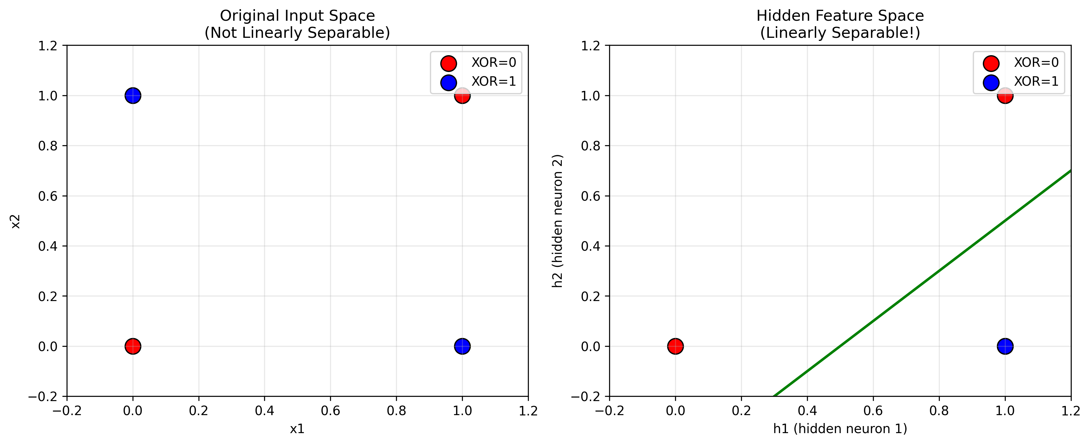
Geometric Interpretation
The hidden layer performs a feature transformation:
- Original space: $(x_1, x_2)$ - XOR is not linearly separable
- Hidden space: $(h_1, h_2)$ - XOR becomes linearly separable.
In the hidden feature space:
- (0,0) maps to [0, 0] - red
- (0,1) maps to [1, 0] - blue
- (1,0) maps to [1, 0] - blue
- (1,1) maps to [1, 1] - red
Now the classes can be separated by the line $h_1 - h_2 = 0.5$.
This is the power of hidden layers: they create new representations where previously impossible problems become solvable.
Why We Can’t Train This Yet
The simple perceptron learning rule outlined at the top of this module only works for single-layer networks.
For multi-layer networks, we face a problem: when the output is wrong, how do we know how much each hidden neuron is “to blame”? How do we update the hidden layer weights?
This is called the credit assignment problem, and it remained unsolved until the invention of backpropagation in the 1980s.
Next module, we’ll learn backpropagation and gradient descent, which allow us to train multi-layer networks automatically.
Resources
Check out these resources if you’re interested in learning more:
-
Interactive TensorFlow Playground
- Try solving XOR with different architectures
- See how hidden layers create feature transformations